Data Science

LuaScript ships a numeric toolkit as native modules: dense N-dimensional arrays, data frames, CSV, statistics, linear algebra, a small neural-network engine, classic clustering and classification algorithms, and a dependency-free SVG plotter. They are all compiled into the interpreter, so require("ndarray") works out of the box with no package manager and no C dependencies.

Module	What it gives you
`ndarray`	Dense N-D arrays over a flat `float64` buffer, NumPy-style broadcasting, overloaded operators, axis reductions, `matmul`
`dataframe`	Column-oriented, pandas-lite tables: `filter`, `with_column`, `sort`, `group_by`, `describe`, CSV in and out
`csv`	Parse and write CSV text and files, with optional header and numeric coercion
`stats`	Descriptive statistics, quantiles, correlation, the normal distribution, t-tests
`linalg`	Vectors and matrices as plain tables: `solve`, `inverse`, `det`, `lstsq`, QR, Cholesky, eigendecomposition
`clustering`	k-means (k-means++ seeding), DBSCAN, hierarchical, mean-shift
`classification`	k-NN, perceptron, logistic regression, SVM (linear and RBF), naive Bayes text classifier
`ml`	Feed-forward neural networks trained by backpropagation, with JSON persistence
`plot`	SVG line, scatter, bar and histogram charts with auto-ranged axes

Each module also has a full offline reference: run luascript doc ndarray, luascript doc dataframe.frame, luascript doc plot.figure, and so on. For the rest of the native modules, see Native modules.

Indices and axes are 1-based everywhere, like the rest of the language. a:sum(1) reduces over the first axis (the rows), giving one value per column.

ndarray

ndarray is a NumPy-shaped array type. You build one from a nested table, and the nesting depth becomes the number of dimensions. Arithmetic operators (+ - * / % ^ and unary -) are overloaded and broadcast, == compares shape and contents, # gives the length of the first axis, and print pretty-prints.

local nd = require("ndarray")
 
local a = nd.array({ {1, 2, 3}, {4, 5, 6} })
print(a)
print(a:shape()[1], a:shape()[2], a:ndim(), a:size())
 
print(a * 2 + 1)                       -- scalar broadcast
print(a + nd.array({10, 20, 30}))      -- row broadcast across both rows
print(-a)

[[1 2 3],
 [4 5 6]]
2	3	2	6
[[ 3  5  7],
 [ 9 11 13]]
[[11 22 33],
 [14 25 36]]
[[-1 -2 -3],
 [-4 -5 -6]]

Broadcasting follows the NumPy rules: trailing dimensions must match or be 1. Mismatched shapes raise an ordinary runtime error:

local nd = require("ndarray")
local ok, err = pcall(function()
  return nd.array({1, 2, 3}) + nd.array({1, 2})
end)
print(ok, err)
--> false	snippet.lsc:3: ndarray:+: operands could not be broadcast together with shapes (3) and (2)

Reductions and matrix products

Reductions take an optional 1-based axis. With no axis they reduce the whole array and return a plain Lua number, not a 0-dimensional array. The same goes for the dot product of two vectors.

local nd = require("ndarray")
local a = nd.array({ {1, 2, 3}, {4, 5, 6} })
 
print(a:sum(), a:mean(), a:max())   -- whole array: plain numbers
print(a:sum(1))                     -- reduce axis 1 -> per-column sums
print(a:mean(2))                    -- reduce axis 2 -> per-row means
 
local b = nd.array({ {7, 8}, {9, 10}, {11, 12} })
print(a:matmul(b))
print(nd.array({1, 2, 3}):dot(nd.array({4, 5, 6})))   -- vectors -> a number

21.0	3.5	6.0
[5 7 9]
[2 5]
[[ 58  64],
 [139 154]]
32.0

Constructors and transforms

local nd = require("ndarray")
print(nd.zeros({2, 2}))
print(nd.arange(0, 5))                  -- [start, stop)
print(nd.linspace(0, 1, 5))             -- [start, stop], n points
print(nd.arange(6):reshape({2, 3}))
print(nd.arange(1, 5):sqrt())
print(nd.array({1, 2, 3, 4}):map(function(x) return x * x end))
 
local a = nd.array({ {1, 2}, {3, 4} })
print(a == a:copy(), a:get(2, 1), #a)

[[0 0],
 [0 0]]
[0 1 2 3 4]
[   0 0.25  0.5 0.75    1]
[[0 1 2],
 [3 4 5]]
[      1 1.41421 1.73205       2]
[ 1  4  9 16]
true	3.0	2

Function	Description
`ndarray.array(t)` / `ndarray.from_table(t)`	Build an array from a nested table
`ndarray.zeros(shape)`, `ndarray.ones(shape)`, `ndarray.full(value, shape)`	Constant-filled array; `shape` is a table such as `{2, 3}`
`ndarray.eye(n)`	The n×n identity matrix
`ndarray.arange([start,] stop [, step])`	Evenly spaced values over `[start, stop)`
`ndarray.linspace(start, stop, n)`	`n` values evenly spaced over `[start, stop]`
`ndarray.matmul(a, b)`	Matrix product; two vectors give their dot product as a number
`ndarray.concat(a, b [, axis])`	Join two 1-D arrays end to end (higher dimensions raise)
`ndarray.is_ndarray(v)`	Whether `v` is an ndarray rather than a plain table

Methods	Description
`a:get(...)`, `a:set(value, ...)`	Read or write one element by 1-based indices
`a:shape()`, `a:ndim()`, `a:size()`	Dimensions, number of dimensions, element count
`a:reshape(shape)`, `a:flatten()`, `a:transpose()`, `a:copy()`	Reshaping (a copy; one dimension may be `-1`) and copying
`a:to_table()`	Back to a nested Lua table
`a:add(b)`, `a:sub(b)`, `a:mul(b)`, `a:div(b)`, `a:neg()`, `a:pow(e)`	Method forms of the operators
`a:matmul(b)`, `a:dot(b)`	Matrix and dot products
`a:sum`, `a:mean`, `a:prod`, `a:min`, `a:max`, `a:std`, `a:var`	Reductions, each taking an optional `axis`
`a:argmin()`, `a:argmax()`	1-based flat index of the smallest / largest element (no axis form)
`a:abs`, `a:sqrt`, `a:exp`, `a:log`, `a:log2`, `a:log10`, `a:sin`, `a:cos`, `a:tanh`, `a:sinh`, `a:cosh`, `a:asin`, `a:acos`, `a:atan`, `a:floor`, `a:ceil`, `a:round`, `a:sign`	Elementwise math
`a:clip(lo, hi)`	Constrain every element to `[lo, hi]`
`a:sort()`, `a:argsort()`, `a:cumsum()`, `a:diff()`, `a:nonzero()`	Ordering and running operations
`a:map(fn)`	Apply a Lua function to every element

For one-off work on small matrices, linalg operates on plain tables instead; ndarray is the faster choice for large or repeated numeric work because it stores one flat buffer rather than a table per row.

dataframe

A data frame is a column-oriented table: each column is a named array, all of the same length. Every transforming method returns a new frame, so calls chain and never mutate the original. Row callbacks receive a table keyed by column name, and print(df) renders an aligned preview.

local dataframe = require("dataframe")
 
local df = dataframe.new({
  name   = { "Ada", "Grace", "Linus", "Margaret", "Dennis" },
  dept   = { "eng", "eng", "eng", "sci", "sci" },
  salary = { 120, 140, 95, 110, 130 },
})
 
local top = df
  :filter(function(row) return row.salary > 100 end)
  :with_column("bonus", function(row) return row.salary * 0.1 end)
  :select({ "name", "salary", "bonus" })
  :sort("salary", true)
print(top)
 
print(df:group_by("dept", { salary = "mean", name = "count" }))
print(df:shape())

name      salary  bonus
--------  ------  -----
Grace     140     14.0
Dennis    130     13.0
Ada       120     12.0
Margaret  110     11.0
dept  salary_mean      name_count
----  ---------------  ----------
eng   118.33333333333  3
sci   120.0            2
5	3

group_by takes a column-to-aggregation table; the aggregations are sum, mean (or avg), min, max, median, std, var, count, first and last. Each output column is named <column>_<aggregation>.

Data that arrives as rows (a query result, a decoded JSON array) goes through from_rows; describe summarises the numeric columns:

local dataframe = require("dataframe")
local df = dataframe.from_rows({
  { name = "ada",   dept = "eng",      salary = 120 },
  { name = "grace", dept = "eng",      salary = 130 },
  { name = "alan",  dept = "research", salary = 110 },
})
print(table.concat(df:columns(), ", "))
print(df:describe())
io.write(df:select({ "name", "salary" }):to_csv())

name, dept, salary
statistic  salary
---------  ------
count      3
mean       120.0
std        10.0
min        110.0
25%        115.0
50%        120.0
75%        125.0
max        130.0
name,salary
ada,120
grace,130
alan,110

Function / method	Description
`dataframe.new(columns)`	Build from a table of named, equal-length columns
`dataframe.from_rows(rows)`	Build from an array of row tables; column names come from the keys
`dataframe.from_csv(path)`	Read a CSV file; the header line names the columns and numeric-looking columns become numbers
`df:col(name)`, `df:row(i)`, `df:rows()`	One column as an array, one row (or all rows) as records
`df:select(names)`, `df:drop(names)`	Keep or remove columns; pass the names as a table
`df:rename(mapping)`	Rename columns from an old-name to new-name table
`df:filter(fn)`, `df:with_column(name, fn)`	Keep rows where `fn(row)` is truthy; add a computed column
`df:sort(name [, descending])`	Order rows by one column
`df:group_by(name, aggs)`	Group and aggregate
`df:head([n])`, `df:tail([n])`	First or last `n` rows (default 5)
`df:shape()`, `df:columns()`, `df:describe()`	Row and column counts, column names, summary statistics
`df:to_csv([path])`	Write to a file, or return CSV text when called with no path

csv

csv reads and writes CSV, handling quoting and embedded delimiters. By default rows are arrays of strings; pass { header = true } to get records keyed by the header, and numbers = true to coerce numeric fields.

local csv = require("csv")
 
local text = "name,age,city\nAda,36,London\nGrace,40,\"New York, NY\"\n"
 
local rows = csv.parse(text)                 -- array of string arrays
print(#rows, rows[3][3])
 
local records = csv.parse(text, { header = true, numbers = true })
print(records[2].name, records[2].age + 1)   -- age is a number
 
io.write(csv.stringify(records, { header = true, columns = { "name", "age" } }))

3	New York, NY
Grace	41
name,age
Ada,36
Grace,40

Function	Description
`csv.parse(text [, opts])`	Parse CSV text in memory
`csv.stringify(rows [, opts])`	Render rows or records as CSV text; `columns` fixes the column order
`csv.read(path [, opts])`	Read a CSV file
`csv.write(path, rows [, opts])`	Write a CSV file

For typed, column-wise work, load the file with dataframe.from_csv instead.

stats

Every stats function takes a plain array of numbers; the relationship functions take two equal-length arrays. Mind the sample/population split: variance and stddev divide by n-1, pvariance and pstddev divide by n.

local stats = require("stats")
local xs = { 2, 4, 4, 4, 5, 5, 7, 9 }
 
print(stats.mean(xs), stats.median(xs), stats.mode(xs))
print(stats.variance(xs), stats.pvariance(xs))   -- sample (n-1) vs population (n)
print(stats.percentile(xs, 90), stats.iqr(xs))
 
local d = stats.describe(xs)
print(d.count, d.mean, d.min, d.q1, d.median, d.q3, d.max)
 
print(stats.correlation({ 1, 2, 3, 4 }, { 2, 4, 6, 8 }))
print(string.format("%.4f", stats.normal_cdf(1.96)))
 
local t = stats.t_test_2sample({ 12, 14, 11, 13, 15, 12 }, { 16, 18, 17, 15, 19, 17 })
print(string.format("t=%.3f p=%.5f", t.t, t.p))

5.0	4.5	4.0
4.5714285714286	4.0
7.6	1.5
8	5.0	2.0	4.0	4.5	5.5	9.0
1.0
0.9750
t=-5.000 p=0.00054

Group	Functions
Central tendency	`mean`, `median`, `mode`, `geomean`, `harmonic_mean`, `weighted_mean(xs, weights)`
Spread	`variance`, `stddev`, `pvariance`, `pstddev`, `sem`, `range`, `iqr`, `min`, `max`
Quantiles	`quantile(xs, q)` with q in `[0, 1]`, `percentile(xs, p)` with p in `[0, 100]`
Shape	`skewness`, `kurtosis`
Aggregates	`sum`, `product`, `cumsum`
Relationships	`covariance`, `correlation` (Pearson), `spearman` (rank)
Transforms	`normalize` (to `[0, 1]`), `standardize` / `zscore` (mean 0, unit variance)
Summary	`describe(xs)` returns `count`, `mean`, `std`, `min`, `q1`, `median`, `q3`, `max`
Distributions	`histogram(xs [, bins])` returns `{ counts, edges }`; `normal_pdf(x [, mu [, sigma]])`, `normal_cdf(x [, mu [, sigma]])`
Tests	`t_test_1sample(xs [, mu])`, `t_test_2sample(xs, ys)`, each returning `{ t, df, p }`

linalg

linalg works on plain tables: a vector is a flat array and a matrix is an array of row arrays, so results interoperate with the rest of your code without wrapping.

local linalg = require("linalg")
 
local A = { { 2, 1 }, { 1, 3 } }
print(linalg.det(A), linalg.trace(A), linalg.rank(A))
 
local x = linalg.solve(A, { 5, 10 })    -- 2x + y = 5, x + 3y = 10
print(x[1], x[2])
 
local inv = linalg.inverse(A)
print(inv[1][1], inv[1][2])
 
print(linalg.dot({ 1, 2, 3 }, { 4, 5, 6 }), linalg.norm({ 3, 4 }))
 
-- least squares: fit y = m*x + c through noisy points
local design, ys = {}, {}
for i = 1, 5 do
  design[i] = { i, 1 }
  ys[i] = 2 * i + 1 + (if i % 2 == 0 then 0.1 else -0.1)
end
local fit = linalg.lstsq(design, ys)
print(string.format("slope %.4f, intercept %.4f", fit[1], fit[2]))

5.0	5.0	2
1.0	3.0
0.6	-0.2
32.0	5.0
slope 2.0000, intercept 0.9800

The jitter above uses an if expression. The c and a or b idiom works too: the checker types cond and 0.1 or -0.1 as number, because a false on the left of or cannot be the result.

Group	Functions
Vectors	`add(a, b)`, `sub(a, b)`, `scale(a, k)`, `dot(u, v)`, `norm(v)`, `distance(u, v)`
Matrices	`matmul(a, b)`, `matvec(a, v)`, `transpose(a)`, `det(a)`, `trace(a)`, `rank(a)`, `inverse(a)`
Solvers	`solve(a, b)` (square, full rank), `lstsq(a, b)` (overdetermined systems)
Decompositions	`qr(a)` returns `Q, R`; `cholesky(a)` returns `L`; `eigh(a)` for symmetric matrices returns eigenvalues and eigenvectors
Constructors	`identity(n)`, `zeros(rows, cols)`, `ones(rows, cols)`

clustering

Unsupervised grouping of points, where a point is an array of coordinates and the data is an array of points. kmeans and meanshift return a table with centroids, assignments (1-based cluster indices, parallel to the input) and, for k-means, iterations. dbscan and hierarchical return the label array directly; DBSCAN labels noise points 0 instead of forcing them into a cluster.

local clustering = require("clustering")
 
local data = {
  { 1.0, 1.0 }, { 1.5, 2.0 }, { 1.3, 1.4 },
  { 8.0, 8.0 }, { 9.0, 8.5 }, { 8.5, 9.0 },
}
 
local km = clustering.kmeans(data, 2, { seed = 1 })
print(table.concat(km.assignments, " "), km.iterations)
print(string.format("centroid 1: (%.3f, %.3f)", km.centroids[1][1], km.centroids[1][2]))
 
-- DBSCAN and hierarchical return the label array directly (0 = noise)
print(table.concat(clustering.dbscan(data, 2.0, 2), " "))
print(table.concat(clustering.hierarchical(data, 2, { linkage = "complete" }), " "))
 
local ms = clustering.meanshift(data, 3.0)
print(#ms.centroids, table.concat(ms.assignments, " "))

2 2 2 1 1 1	2
centroid 1: (8.500, 8.500)
1 1 1 2 2 2
1 1 1 2 2 2
2	1 1 1 2 2 2

The signatures are type-checked against what each function really takes, options table included. Leaving out DBSCAN's min_pts, for example, is a compile error:

local clustering = require("clustering")
local labels = clustering.dbscan({ { 1, 1 }, { 2, 2 } }, 2.0)

luascript: call passes 2 args, function expects at least 3 at line 2

Function	Description
`clustering.kmeans(points, k [, opts])`	Lloyd's algorithm with k-means++ seeding; options include `seed`, `maxIter`, `delta`
`clustering.dbscan(points, eps, min_pts)`	Density-based: discovers the cluster count, labels noise `0`
`clustering.hierarchical(points, k [, opts])`	Agglomerative, merging until `k` clusters remain; `linkage` option such as `"complete"`
`clustering.meanshift(points, bandwidth [, opts])`	Mode-seeking; the bandwidth controls how many clusters emerge

classification

Supervised classifiers. The numeric models (knn, perceptron, logistic, svm) share a :fit(features, labels) / :predict(x) interface, where features is an array of coordinate arrays and labels can be any values. naivebayes is text-oriented and works on token lists instead.

local classification = require("classification")
 
local features = {
  { 1.0, 1.0 }, { 1.5, 2.0 }, { 2.0, 1.5 },
  { 8.0, 8.0 }, { 9.0, 8.5 }, { 8.5, 9.0 },
}
local labels = { "A", "A", "A", "B", "B", "B" }
 
local knn = classification.knn(3)
knn:fit(features, labels)
print(knn:predict({ 1.2, 1.3 }), knn:predict({ 8.7, 8.2 }))
 
local lr = classification.logistic({ lr = 0.5, epochs = 500 })
lr:fit(features, labels)
print(lr:predict({ 7.5, 8.0 }), string.format("%.4f", lr:predict_proba({ 7.5, 8.0 })))
 
local svm = classification.svm({ kernel = "linear", C = 1.0 })
svm:fit(features, labels)
print(svm:predict({ 2, 2 }), string.format("%.3f", svm:decision_function({ 2, 2 })))
 
-- Naive Bayes works on token lists
local nb = classification.naivebayes("spam", "ham")
nb:learn({ "buy", "cheap", "pills", "now" }, "spam")
nb:learn({ "lunch", "meeting", "tomorrow" }, "ham")
print((nb:classify({ "cheap", "buy" })))

A	B
B	0.9919
A	-0.920
spam

Constructor	Model methods
`classification.knn([k])`	`:fit`, `:predict`; `k` defaults to 3
`classification.perceptron([opts])`	`:fit`, `:predict`; options `lr`, `epochs`
`classification.logistic([opts])`	`:fit`, `:predict`, `:predict_proba`; options `lr`, `epochs`
`classification.svm([opts])`	`:fit`, `:predict`, `:decision_function`, `:support_vectors`; options `kernel` (`"rbf"`, the default, `"linear"` or `"poly"`), `C`, `gamma`, `coef0`, `degree`, `tol`, `maxIter`, `seed`; `:support_vectors()` returns the count
`classification.naivebayes(class, ...)`	`:learn(tokens, class)`, `:classify(tokens)`, `:classifyProb(tokens)`, `:classes()`, `:learned()`

nb:classify returns three values: the winning class, the per-class scores, and whether the decision was strict (no tie). nb:classifyProb returns the class and an array of probabilities in class order.

ml

ml is a small feed-forward neural-network engine trained by backpropagation. ml.new takes a topology and hyperparameters; net:train takes the training data and solver settings; net:predict runs a forward pass and returns the output layer as an array.

local ml = require("ml")
 
-- XOR: 2 inputs -> 4 tanh hidden units -> 1 sigmoid output
local net = ml.new({
  inputs     = 2,
  layout     = { 4, 1 },
  activation = "tanh",
  mode       = "binary",
  bias       = true,
  weight     = { kind = "normal", stddev = 0.5 },
})
 
local data = {
  { input = { 0, 0 }, response = { 0 } },
  { input = { 0, 1 }, response = { 1 } },
  { input = { 1, 0 }, response = { 1 } },
  { input = { 1, 1 }, response = { 0 } },
}
 
net:train({
  data       = data,
  iterations = 2000,
  solver     = { kind = "adam", lr = 0.05 },
})
 
for _, ex in ipairs(data) do
  local out = net:predict(ex.input)
  print(ex.input[1], ex.input[2], math.floor(out[1] + 0.5))
end
 
-- marshal/load round-trips through a JSON string; save/load_file through a file
local restored = ml.load(net:marshal())
print(restored:num_weights() == net:num_weights())

Weights are initialised randomly and there is no seed option, so exact outputs vary from run to run; on rare runs a tiny network like this one can settle in a poor local minimum.

Function / method	Description
`ml.new(config)`	Create a network. `config` keys: `inputs`, `layout` (layer sizes, last is the output), `activation`, `mode` (for example `"binary"` for a sigmoid output), `bias`, `weight`
`net:train(opts)`	Train; `opts` keys: `data` (array of `{ input, response }`), `validation`, `iterations`, `solver` (for example `{ kind = "adam", lr = 0.05 }`), `verbosity` (print loss every N epochs)
`net:predict(input)`	Forward pass; returns the output layer
`net:marshal()` / `ml.load(blob)`	Serialise to a JSON string and restore
`net:save(path)` / `ml.load_file(path)`	The same, through a file
`net:num_weights()`, `net:weights()`	Weight count, and the weights as a nested table per layer

plot

plot renders charts to standalone SVG with no external dependencies: no fonts to install, no headless browser. Axes are auto-ranged onto "nice" 1-2-5 ticks, and a legend appears as soon as a series has a label.

There are two ways in. plot.figure([opts]) gives you an empty canvas to add several series to; plot.line, plot.scatter, plot.bar and plot.histogram build a one-series figure in a single call. Every figure method returns the figure, so calls chain.

The four charts below are produced by 48_plot_module.lsc. The first is a multi-series figure: a line and a scatter sharing axes, with options passed as tables.

line.lsc

local plot = require("plot")
 
local xs, sq, noisy = {}, {}, {}
for i = 1, 20 do
  xs[i] = i
  sq[i] = i * i
  noisy[i] = i * i + (i % 3 - 1) * 12   -- deterministic wobble
end
 
local fig = plot.figure({ title = "y = x^2", xlabel = "x", ylabel = "y", width = 720, height = 420 })
fig:line(xs, sq, { label = "exact", color = "#4e79a7" })
   :scatter(xs, noisy, { label = "observed", color = "#e15759" })
fig:save("plot-line.svg")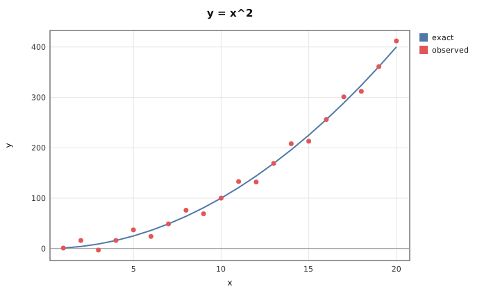

plot.figure with a line series and a scatter series sharing auto-ranged axes

The one-call constructors cover the single-series cases:

charts.lsc

local plot = require("plot")
 
plot.bar({ "apple", "pear", "plum", "fig" }, { 8, 5, 3, 6 })
  :title("fruit counts"):ylabel("count")
  :save("plot-bar.svg")
 
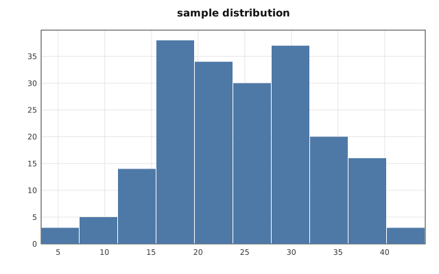
-- the mean of three uniform draws is bell-shaped; a tiny LCG keeps it deterministic
local seed = 12345
local function uniform()
  seed = (seed * 1103515245 + 12345) % 2147483648
  return seed / 2147483648
end
local samples = {}
for i = 1, 200 do samples[i] = (uniform() + uniform() + uniform()) / 3 * 50 end
plot.histogram(samples, 10):title("sample distribution"):save("plot-hist.svg")
 
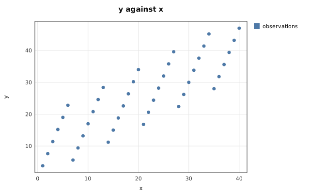
local px, py = {}, {}
for i = 1, 40 do
  px[i] = i
  py[i] = i * 0.8 + (i % 7) * 3
end
plot.scatter(px, py, "observations")
  :title("y against x"):xlabel("x"):ylabel("y")
  :save("plot-scatter.svg")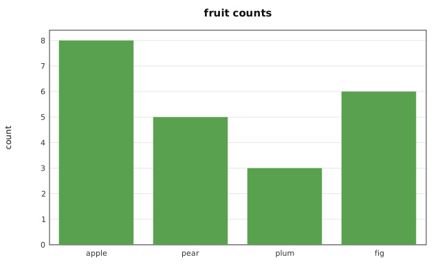

plot.bar: labelled categories (fruit counts)

plot.histogram: 200 bell-shaped samples in 10 bins

plot.scatter: 40 points around a linear trend

Function / method	Description
`plot.figure([opts])`	Empty figure; `opts` may set `title`, `xlabel`, `ylabel`, `width`, `height`
`plot.line(xs, ys [, label])`	Ordered series: time, a sweep, a trend
`plot.scatter(xs, ys [, label])`	Unordered pairs: correlation, clusters
`plot.bar(labels, values [, label])`	Labelled categories
`plot.histogram(values [, bins [, label]])`	One series, binned: the shape of a distribution
`fig:line`, `fig:scatter`, `fig:bar`, `fig:histogram`	Add a series; the last argument is a label string or an options table with `label` and `color`
`fig:title(s)`, `fig:xlabel(s)`, `fig:ylabel(s)`, `fig:size(w, h)`	Set titles and output size in pixels
`fig:to_svg()`	Render and return the SVG text, to embed or serve
`fig:save(path)`	Render and write to a file

Putting it together

The modules interoperate through plain tables, so a CSV-to-chart pipeline is a few lines:

local dataframe = require("dataframe")
local stats = require("stats")
local plot = require("plot")
 
local f = io.open("cities.csv", "w")
f:write("city,population\nOslo,709000\nBergen,286000\nTromso,77000\n")
f:close()
 
local df = dataframe.from_csv("cities.csv")      -- numeric columns come back as numbers
local pops = df:col("population")
print("mean:", stats.mean(pops), "median:", stats.median(pops))
 
plot.bar(df:col("city"), pops, "population")
  :title("Norwegian cities")
  :save("cities.svg")

mean:	357333.33333333	median:	286000.0

Examples

File	What it shows
`47_ndarray_module.lsc`	Construction, broadcasting, reductions, matmul, concat
`40_dataframe_module.lsc`	select/filter/with_column/sort/group_by/describe, rows and CSV
`39_csv_module.lsc`	Parsing, header and numeric coercion, file round trip
`37_stats_module.lsc`	The full statistics surface, including histograms and t-tests
`38_linalg_module.lsc`	Solvers, least squares, QR, Cholesky, eigendecomposition
`34_clustering_module.lsc`	k-means, DBSCAN, hierarchical, mean-shift
`35_classification_module.lsc`	Naive Bayes, k-NN, perceptron, logistic regression, linear and RBF SVM
`41_ml_module.lsc`	Training XOR, prediction, persistence
`48_plot_module.lsc`	All four chart types